on
MNIST handwritten digit recognition: A comparison between One-vs-All from scratch and One-vs-All from scikit-learn
This is a documentation of my steps in building a one-vs-all learning algorithm from scratch and its performance on the MNIST handwriting dataset. I will then use the most similar algorithm available in scikit-learn library and we’ll take a look at the pros and cons of each.
The motivation for this project is for me to walk through the logic and math of this algorithm. I like to connect the dots of the details of the algorithms I use, and the most concrete way to do this is to build it from scratch. However, many machine learning packages are written with greater considerations of different models and optimizations. It is unfeasible and unecessary to write algorithms that are as good or better than available existing libraries that have been constructed with thought and care by experts. So this project serves a second purpose: to understand the options available and how to use scikit-learn to obtain equal or better results once I understand the basics of the algorithm.
The challenge
The MNIST dataset is a well known dataset to learn about image classification or just classification in general. It contains handwritten digits from 0 to 9, 28x28 pixels in size. Our task is to train a model that will be able to take an image as input and predict the digit on that image.
The dataset used for this post is downloaded from Kaggle. But it is available in many different places as well. In this dataset, each row is a sample. One column is the label, which tells us the digit of the sample (0-9). The rest of the columns are intensities of the pixels of the image. So we have 28 x 28 = 784 columns of pixel intensities.
These are some examples of the images:
import matplotlib as plt
import pandas as pd
import numpy as np
import seaborn as sns # optional. Makes matplotlib more visually pleasing.

MNIST = pd.read_csv("train.csv")
images = []

# populate images with the first occuring samples of each digit, convert
# pandas dataframe to numpy arrays so that they can be plotted as images
for i in range(10):
    a = MNIST.loc[MNIST.loc[:, "label"] == i, ]
    a = a.loc[a.index[0], ]
    a = a[1:, ]
    a = a.values
    a = a.reshape(28, 28)
    images.append(a)

fig, ax = sns.plt.subplots(2, 5)
n = 0
for r in range(2):
    for c in range(5):
        ax[r, c].imshow(images[n])
        ax[r, c].axis("off")
        n += 1
sns.plt.savefig("images.png", bbox_inches="tight", pad_inches = 0)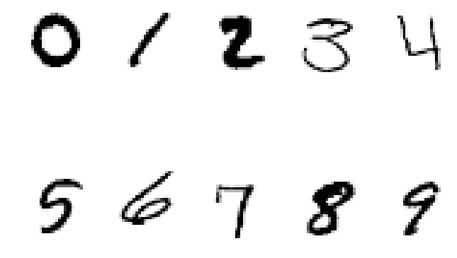
Because we have more than one feature, we also need to standardize them, or gradient descent will take forever to converge, if it converges at all.
def standardize(inputdata, columns):
    """ data is a pandas dataframe to be standardized
columns is a list of column names to be standardized.
Returns a dataframe where values are standardized by:
((value-mean)/range)."""
    data = copy.deepcopy(inputdata)
    for i in columns:
        imean = sum(data[i])/len(data[i])
        if imean == 0:
            continue
        irange = max(data[i])-min(data[i])
        data[i] = (data[i]-imean)/irange
    return data

featureCols = [i for i in MNIST.columns[1:]]

mnist = standardize(MNIST, featureCols)
For each image, there are a lot of pixels that likely remain empty/white for all samples. This can be confirmed when you run MNIST.describe(). These pixels/features can be removed because they remain constant in the dataset, thus will have no predictive impact on the model. We can remove the pixels that have a standard deviation of 0. Meaning there is no variation in pixels of this location in the entire training set.
mnistSumStats = mnist.describe()
mnist = mnist.loc[:, mnistSumStats.loc["std",] != 0]

# this takes a while to compute, so save and load later.
mnist.to_csv("mnistClean.csv", index = False)
Logistic Regression One-vs-All from scratch
Logistic regression is used for binary classification. The hypothesis function in logistic regression takes in x-values (the features), and outputs a y-value (prediction) between 0 and 1. With 1 being positive and 0 being negative.
In this case, an x value will be the intensity of a pixel at a specific location, and y value would be 0 or 1.
The hypothesis calculation:
def hypothesis(X, theta):
    """ Takes X and theta and returns the hypothesis
for logistic regression (sigmoidal curve).
X - numpy matrix of shape x, j
theta - numpy matrix of shape k, j
where x is the number of samples,
j is the number of features,
k is the number of y-values.
returns a matrix of shape x, k."""
    return 1/(1+np.exp(-(X*theta.T)))
How can we classify our dataset into 10 categories if logistic regression only classifies into two groups (0 or 1)? One-vs-All means we train 10 models, one for each digit. For example, to classify 5, the model will treat all other digits as one class and digits 5 as another. It would output a value close to 1 if it predicts an image to be 5 and 0 if it predicts and image to be not 5. This is written after going through Andrew Ng’s Machine Learning lectures on one-vs-all logistic regression.
To be able to train these models, we need to classify our samples into 10 labels of 0’s and 1’s instead of 0 to 9.
Processing y-values so that it is a 1x10 vector of 0’s and 1’s:
mnist = pd.read_csv("mnistClean.csv")

def setUpY(data, Ycolumn, Yvalue):
    res = copy.deepcopy(data)
    return (res.loc[:, Ycolumn] == Yvalue)*1

for i in range(10):
    mnist[str(i)] = setUpY(mnist, "label", i)
This results in the following:
mnist.iloc[:, 709:].head() 0 1 2 3 4 5 6 7 8 9
0 0 1 0 0 0 0 0 0 0 0
1 1 0 0 0 0 0 0 0 0 0
2 0 1 0 0 0 0 0 0 0 0
3 0 0 0 0 1 0 0 0 0 0
4 1 0 0 0 0 0 0 0 0 0To train 10 models in one go, it will be much easier to use numpy matrices and linear algebra than to do it iteratively. As the hypothesis function is written for numpy matrices, we can easily scale this up to 10 models.
Right now, we have reduced the number of features to 709 by removing pixels with no variations. Our label has gone from 1 column to 10 columns by generating the 0 and 1 matrices. We have 42000 rows in our training data downloaded from Kaggle. Therefore, X is now a 42000 x 709 matrix. Y is a 42000 x 10 matrix. For theta to multiply X and get a matrix that has the same dimension as Y, it has to be a 10 x 709 matrix. It may be easier to have it as a 709 x 10 matrix, but because of how I set up my code when I used it for binary classification (and so theta was only a vector rather than a matrix), it’s easier for me to change the dimension of theta.
Of course, our next step is to split the dataset into train, validation, and test set. This will change the shapes of our X and Y matrices but you can work out that it will not affect the shape of theta.
Here’s a really bad, throwaway function that will split the data into train, validation, and test sets. Split the data after processing the y-values, dropping the original “label” column, and adding a column of x0 (values of 1).
mnist.insert(1, "x0", 1) # insert x0
mnist = mnist.iloc[:, 1:] # drop the "label" column

def splitData(data, trainpc, validpc):
    """given a data frame, returns
training, validation, test sets that are shuffled."""
    np.random.seed(10101)
    shuffled = data.reindex(np.random.permutation(data.index))
    totrows = data.shape[0]
    trainsize = int(trainpc*totrows)
    validsize = int(validpc*totrows)+trainsize
    return shuffled[:trainsize], shuffled[trainsize:validsize], shuffled[validsize:]

train, validation, test = splitData(mnist, 0.8, 0.1)
We are now almost ready to go. We just need a cost function to optimize and a function to update theta values while doing gradient descent/ascent. Because this is logistic regression, the cost function is the log likelihood function. You can put a negative to this function so it decreases to 0 rather than increase to 0, but it really is the same thing:
# regularization is not done to theta0, so these are the functions to separate
# theta into theta0 and thetaj for subsequent calculations.
def splitTheta(theta):
    theta0, thetaj = np.split(theta, [1], axis = 1)
    return theta0, thetaj

def joinTheta(theta0, thetaj):
    return np.concatenate((theta0, thetaj), axis = 1)

# log likelihood. To be maximized. (with regularization term)
def logllhood(X, y, theta, lmb):
    theta0, thetaj = splitTheta(theta)
    res = np.log(hypothesis(X, theta)).T*y+np.log(1-hypothesis(X,theta)).T*(1-y)-(lmb/2)*thetaj*thetaj.T
    return res.diagonal()

# You can think of this as gradient descent if you put a negative to the log
# likelihood. It achieves the same goal, we're just flipping values across the x-axis.
def gradientAscent(X, Xj, y, theta, x0, alpha, lmb):
    theta0, thetaj = splitTheta(theta)
    theta0 = theta0*(1- alpha*(lmb/len(X))) + alpha*(1/len(X))*((y-hypothesis(X, theta)).T*x0)
    thetaj = thetaj*(1- alpha*(lmb/len(X))) + alpha*(1/len(X))*((y-hypothesis(X, theta)).T*Xj)
    theta = joinTheta(theta0, thetaj)
    return theta
Because this dataset is rather large, I’m hesitant to do batch gradient descent/ascent. Instead I’ve decided to implement mini batch gradient descent.
Batch gradient descent does a calculation with the entire training set and returns a new theta value. Stochastic gradient descent does a calculation with a single sample and updates the theta value. Mini batch gradient descent does a calculation with a subset of the dataset, and updates the theta value. So it’s a compromise of the batch and stochastic gradient descent.
To do this, we just have to split our training set up into mini batches. Here, I’ve done the math and a mini batch of 4200 is splitting the training data into eight equal batches. However, there’s no need to keep it equal in size if you don’t want to, everything still works. I just want to prevent missing data because of the way numbers and division work in python.
def makeMiniBatches(data, miniBatchSize):
    """Shuffles and makes data into a list of minibatches
of length x. """
    x = int(data.shape[0]/miniBatchSize)
    shuffled = data.reindex(np.random.permutation(data.index))
    totX = np.matrix(shuffled.values)
    return np.array_split(totX, x)
We are now ready to construct the main loop. This will be the function that gets our model to go through the dataset in mini batches until convergence.
def mainLoop(trainingset, miniBatchSize, alpha, lmb, iters, numberOfLabels):
    miniBatches = makeMiniBatches(trainingset, miniBatchSize)
    X = np.matrix(trainingset.values)
    X, Y = np.split(X, [709], axis = 1)
    x = len(miniBatches)
    n = 0
    i = 0
    theta = np.matrix( [[0]*709]*numberOfLabels )
    logll = [[] for i in range(numberOfLabels)]
    iterations = []
    while n <= iters:
        if (i+1)%x == 0:
            miniBatches = makeMiniBatches(trainingset, miniBatchSize)
            i = 0
        mini = miniBatches[i]
        Xmini, Ymini = np.split(mini, [709], axis = 1)
        x0, xj = np.split(Xmini, [1], axis = 1)
        theta = gradientAscent(Xmini, xj, Ymini, theta, x0, alpha, lmb)
        if n%100 == 0:
            iterations.append(n)
            err = logllhood(X, Y, theta, lmb)
            for p in range(len(logll)):
                logll[p].append(err[0, p])
            print(n)
            print(err)
        n += 1
        i += 1
    return theta, logll, iterations
This function does the following:
- Makes a list of pandas dataframe of
miniBatchSizefrom training data. - Makes
XandYmatrices from training data. (for log likelihood calculations) - Goes through mini batches after mini batches for
itersnumber of times, updatingthetaat every iteration. - Reports and records the log likelihood every 100 iterations. This helps us plot the cost function later on. The reporting is for your sanity.1
We are now ready to train!
It’s good to have a bit of a system set up while training. I like to look at the cost function (it’s called error in this code) over number of iterations. This is a great check to be sure that your alpha value is not so large that your model has overshot the minimum (gradient descent) or maximum (gradient ascent). By having the loop report the errors every 100 iterations, we can also check that the values make sense. In this case, log likelihood starts from a huge negative number and approaches 0 asymptotically. So if it does something weird like shoot up to positive values, the math is wrong somewhere. Terminate and find the bug.
If the model is not working as you had hoped, you can also do many other different types of plots to debug the model or figure out what hyperparameters can be tweaked to make it better. I won’t be doing those here because they weren’t necessary. I also look at the accuracy on the training set and the accuracy on the validation set.
alpha = 10
lmb = 0
iters = 6000

theta, logll, iterations = mainLoop(train, 4200, alpha, lmb, iters, 10)

error = pd.DataFrame(logll)
error = error.transpose()
error["iterations"] = iterations
error = pd.melt(error, id_vars = "iterations", value_vars = [i for i in range(10)])
error["value"] = abs(error["value"])

g = sns.lmplot(x = "iterations",
               y = "value",
               hue = "variable",
               data = error,
               fit_reg = False,
               legend = False)
sns.plt.legend(loc = "upper right")
g.set(yscale = "log")
sns.plt.savefig("80percenttraininglambda"+str(lmb)+"alpha"+str(alpha)+"iter"+str(iters)+".png")

# predict
def predict(data, theta):
    X = np.matrix(data.values)
    X, Y = np.split(X, [709], axis = 1)
    predictedVal = hypothesis(X, theta)

    predictedNum = np.argmax(predictedVal, axis = 1)
    actualNum = np.argmax(Y, axis = 1)

    accuracy = sum(actualNum == predictedNum)/actualNum.shape[0]

    df = pd.DataFrame({"actual" : actualNum.tolist(), "predicted" : predictedNum.tolist()})
    df["accuracy"] = (df.loc[:, "actual"] == df.loc[:, "predicted"])*1

    return float(accuracy), df

train_accur, trainpd = predict(train, theta)
valid_accur, validpd = predict(validation, theta)

import pickle
f = open("alpha"+str(alpha)+"lambda"+str(lmb)+"iter"+str(iters)+".pckl", "wb")
pickle.dump([theta, error, train_accur, trainpd, valid_accur, validpd], f)
f.close()
This way, everytime we finish training, we have several things to look at and decide if we should train again and if so, with what changes.
After training for several alpha values (starting from a conservative 0.01), 10 appears to be the best and 6000 iterations is quite good for having comparable accuracy in training and validation sets.
>>> train_accur
0.9355357142857142
>>> valid_accur
0.919047619047619
Here is the cost function at 6000 iterations. I’ve plotted the absolute values for ease of plotting on a log scale (just laziness to read the docs and figure out how to do negative log scale).
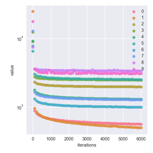
This is a very interesting plot as you can see which digits have models that produce better predictions. 8 and 9 suffer from a high error compared to models for 1 and 0. Apparently, some digits are easier to read than others! This makes sense as there are variations in how digits are written, but some digits, such as 0 and 1, have less variations. Different models also converge at different rates. Models for 8 and 9 clearly converged much earlier than models for 0 and 1.
Now that I’m satisfied with the error rates and accuracy in training and validation sets, let’s see how it does with the test set:
>>> test_accur, testpd = predict(test, theta)
>>> test_accur
0.9154761904761904
This is fairly good! It’s close to our validation accuracy, so we don’t have too big of a overfitting/underfitting problem.
Logistic Regression One-vs-All with scikit-learn
Now let’s see how scikit-learn compares. From the documentation, I compared the different algorithms and functions available. I determined the function most similar to my implementation of the One-vs-All is the LogisticRegression with L2 penalized and using liblinear solver.
It’s important to note that the documentation and tutorial clearly states that this is not the best multiclass classification to use within the library and even within logistic regression classifiers. The purpose of using this classifier is to do a comparison between the method I wrote and how I would be able to implement something similar with scikit learn.
Using the tutorial on scikit learn, I was able to feed the same training and validation sets into the model as I used for my own model:
import pandas as pd
import numpy as np
import matplotlib as plt
import seaborn as sns
import copy as copy
from sklearn.linear_model import LogisticRegression

mnist = pd.read_csv("mnistClean.csv")

def splitData(data, trainpc, validpc):
    """given a data frame, returns
training, validation, test sets that are shuffled."""
    np.random.seed(10101)
    shuffled = data.reindex(np.random.permutation(data.index))
    totrows = data.shape[0]
    trainsize = int(trainpc*totrows)
    validsize = int(validpc*totrows)+trainsize
    return shuffled[:trainsize], shuffled[trainsize:validsize], shuffled[validsize:]

train, validation, test = splitData(mnist, 0.8, 0.1)

Y, X = np.split(train.values, [1], axis = 1)
Yv, Xv = np.split(validation.values, [1], axis = 1)

Y = np.ravel(Y)
Yv = np.ravel(Yv)

model = LogisticRegression( C = 10/train.shape[0],
                            penalty = "l2",
                            solver = "liblinear",
                            max_iter = 6000,
                            verbose = 1)
model.fit(X, Y)
train_accur = model.score(X, Y)
valid_accur = model.score(Xv, Yv)
I used my own functions for splitting the data because I wanted to feed it the exact same train, validation, and test sets. But will definitely explore scikit’s train_test_split() in the future.
>>> train_accur
0.8433630952380953
>>> valid_accur
0.8404761904761905
It has a lower accuracy than the model we wrote from scratch. However, it produced a model in less than a minute. I trained the model I wrote for about 15 minutes for 6000 iterations, which is quite costly as I trained it several times before finding the best hyperparameters.
Conclusion
The one-vs-all logistic regression is a better multiclass model than I originally thought it would be. In fact, with the model I wrote from scratch, when I first ran it with alpha = 0.01 and 1000 iterations, it had an accuracy of 84%.
Scikit learn has a huge library of machine learning algorithms that is worth learning. Acquiring high accuracy requires a good understanding of the tools in this library and how to tweak and evaluate the performance of the models.
Finally, I used the trained model on the Kaggle test set and got a score of 0.91371. This is further confirmation that the model was not overfitted as it closely resembles the accuracy on the validation data.
Footnotes
1Have you ever left your computer on overnight to read in large datasets? Or started making a phylogenetic tree at work and wonder when it’s going to finish so you can pack your laptop and go home? Yea. Silent and slow programs are awful because they can take up to hours to complete and you’ve committed so many hours that you don’t want to terminate it but deep down inside you can’t help but suspect it’s actually crashed and died or an error message is going to pop up anytime. So do yourself a favour, put in a print statement if you think it’s going to take a while, and always look for VERBOSE options when using programs.↩