on
Authorship Prediction in Sci-Fi Literature Part III: N-grams and Word embedding
Part 2 was a lot of exploration in feature engineering and evaluating our choices with the Bag of Words model trained on a simple neural network.
Here in part 3, we’re going to switch gears almost completely and employ word embedding.
Word Embeddings
Word embedding a way to represent words to machine learning models, like Bag of Words. The advantage word embedding has over Bag of Words is that a dataset with 21 thousand unique words, and so 21 thousand unique features can be reduced to having a lot less number of features. Usually the length of the longest sentence is the minimum number of features. Without needing to throw words away like we were doing in the last post.
In essence, we first represent each unique vocabulary word as a unique integer. And every sentence is converted into arrays of integers that represent a word in the vocabluary, and padded to the length of the longest array. So one sentence is converted to a 1xN array, where N is the length of the longest sentence and each element in the array is an integer representing a unique word. Now, we add an embedding layer to our neural network. This layer converts this 1xN array into a NxE matrix, where E is the embedding dimension that can be arbitrarily set. Each unique word is represented by a 1xE vector in this matrix. The 1xE vector is a result of the embedding layer, whose weights can be trainable or pretrained. So each sentence ends up being a two dimensional data type at the end of the embedding layer. We can then process this matrix (summing, averaging, minimum, maximum, concatenation, etc.) into a one dimensional array, and feed it into the next layer.
This is the breakthrough that got my model to hit 80% accuracy. Since we avoid the going through the intermediate 4GB bag of words dataset, we also avoid the big data problem. This is even easier to implement than the Bag of Words method despite the initial complexity of the concept. And since there is a huge reduction in features (from 21k to about 300), we can add new features such as n-grams.
N-grams
N-grams is an Natural Language Processing (NLP) concept. A gram is a word, a single word is known as unigram while two words are known as bigrams. You can go up to 2-gram (bigram), trigram, and so on. For example:
"This is a sample sentence."

Unigrams: "This", "is", "a", "sample", "sentence", "."
Bigrams: "This--is", "is--a", "a--sample", "sample--sentence", "sentence--."
Bigram is a short sequence that may reveal writing style, just like some authors may prefer certain words (the main idea behind Bag of Words), they may also prefer some sequences over others. A simple bigram that can be quite distinctive is “I–said”, or “said–I”. By including bigrams, we capture these features that we would otherwise miss.
More text processing details
Even with word embedding, there are choices to make about feature processing. But we have a greater level of freedom as we are less limited by memory. These are the choices I made and experimented with:
Any word that contains a digit from 0 to 9 is treated as the word “NUMBERS”
The reason I change every string containing a digit to “NUMBERS” is because of the authors in this dataset, I think Jules Verne really likes his numbers written as digits. And how often an author chooses to use digits rather than words to convey numbers may be an identifying feature. I don’t handpick features by looking at the dataset, in fact, I haven’t even looked at it. The only evaluations I’ve done are the distributions of frequency we looked at in the Part 2. This is just something I happen to know about Jules Verne because I’ve read him before.
Stemming
Depending on the size of the dataset, stemming may or may not have a negative effect on model performance. It may oversimplify features or reduce unnecessary features. I don’t think it would have been feasible to try no stemming in the Bag of Words model, but it’s certainly feasible here. Interestingly, not stemming and not converting every word to lowercase boosted performance very slightly (<1%, hey, it’s significant if you’re playing on Kaggle, and a 10% boost is the result of many many tiny boosts). Here are the tokenizers I used:
import pandas as pd
import numpy as np
import nltk # just in case, I'm never quite sure what nltk requires
from nltk.tokenize import TreebankWordTokenizer
from nltk.stem import SnowballStemmer

# Tokenizer for stemming. Stemming converts grams to lowercases
class Snowball():
    def __init__(self):
        self.snow = SnowballStemmer("english")
    def __call__(self, doc):
        return [self.snow.stem(t) for t in TreebankWordTokenizer().tokenize(doc)]

# Tokenizer + lowercase processing
class Treebank():
    def __init__(self):
        self.tree = TreebankWordTokenizer()
    def __call__(self, doc):
        return self.tree.tokenize(doc.lower())

# To tokenize without lowercase, use TreebankWordTokenizer().tokenize
Every gram in training set gets a unique integer, new grams in validation/test sets are treated as the word “UNK” for unknown unigram and “UNKBI” for unknown bigram
The "UNK" and "UNKBI" is a necessary thing to introduce in the validation set. We will always run into words we did not encounter in the training set. However, at the same time, because we did not train with those words, does it cloud our model? Is it better to remove the words completely and have shorter sentences? I think both conditions send the wrong signal to the model. So I decided to treat "UNK" and "UNKBI" as rare unigrams and bigrams rather than unknown unigrams and bigrams. This at least retains some meaning for the model and we will be able to train on these words from our training set. I set a different treshold for unigrams and bigrams because bigrams are less likely to repeat themselves. I ended up replacing unigrams used <= 2 times in the dataset as "UNK" and bigrams used <= once as "UNKBI". This significantly reduced vocabulary size (from about 200k to 50k) and gave me a 1% boost in accuracy.
Implementation
With these modifications, prediction accuracy is about 82% for the validation data. Hyperparameters tuning really doesn’t play a big role in this dataset/neural network model, regularization reduced accuracy of both training and validation set. Here are the functions to implement these processings and sentence arrays to feed into the embedding layer of the neural network:
# import numpy, pandas, and nltk required for tokenizers

def is_a_number(word):
    """ Returns true if word contains a digit."""
    return any(char.isdigit() for char in word)

def convert_to_np_with_padding(array, maxlen):
    """ takes an array and the intended length of array (maxlen)
returns padded array to the length specified.

length of array must be shorter than maxlen."""
    np_array = np.array(
        [np.pad(
            np.array(u),
            (0, max(
                [maxlen-np.array(u).shape[0], 0])),
            "constant",
            constant_values = (0)) for u in array])
    return np_array


def sentences_to_unigram_bigram_arrays_remlowfreq(
    sentences,
    tokenizer):
    """ Turns sentences into unigram and bigram arrays
        to use as input for word embedding. Grams that occur
        <= 2 times are replaced with "UNK" if it's a unigram,
        "UNKBI" if it's a bigram.

        To be used on training set.

        takes the following:
            sentences : {list} of sentences
            tokenizer : a tokenizer
        returns:
            grams_to_int : {dictionary} with grams as
                            keys and integers as values
            vocab_size : {integer} vocabulary size
            unigram array : {numpy array} a sentence encoded with
                            unique index for each word, padded
                            to the length of the longest sentence in sentences.
            bigram array : {numpy array} a sentence encoded with
                            unique index for each bigram, padded to
                            the length of the longest sentence's bigram array."""

    ucounter = {}
    bcounter = {}
    unigrams = []
    bigrams = []
    uni_maxlen = 0
    bi_maxlen = 0
    report = 0
    for s in sentences:
        if report % 1000 == 0:
            print(f"Processing sentence number {report}.")
        s = tokenizer(s)
        uni_array = []
        bi_array = []
        for i in range(len(s)):
            if is_a_number(s[i]):
                s[i] = "ISANUMBER"
            try:
                ucounter[s[i]] += 1
            except KeyError:
                ucounter[s[i]] = 1
            uni_array.append(s[i])
            if i < len(s)-1:
                if is_a_number(s[i+1]):
                    s[i+1] = "ISANUMBER"
                bigram = s[i]+"~~"+s[i+1]
                try:
                    bcounter[bigram] += 1
                except KeyError:
                    bcounter[bigram] = 1
                bi_array.append(bigram)
        unigrams.append(uni_array)
        bigrams.append(bi_array)
        uni_maxlen = max([len(uni_array), uni_maxlen])
        bi_maxlen = max([len(bi_array), bi_maxlen])
        report += 1

    grams_to_int_l = [ugrams for ugrams in ucounter] + [bgrams for bgrams in bcounter] + ["UNK"] + ["UNKBI"]

    print("starting to remove low frequency words.")

    for ucount in ucounter:
        if ucounter[ucount] <= 2:
            grams_to_int_l.pop(grams_to_int_l.index(ucount))

    print("removed low frequency unigrams.")

    for bcount in bcounter:
        if bcounter[bcount] <= 1:
            grams_to_int_l.pop(grams_to_int_l.index(bcount))

    print("removed low frequency bigrams.")

    grams_to_int = {grams_to_int_l[i] : i+1 for i in range(len(grams_to_int_l))}
    print("created dictionary.")

    # replacing grams with integers
    for i in range(len(unigrams)):
        for u in range(len(unigrams[i])):
            try:
                unigrams[i][u] = grams_to_int[unigrams[i][u]]
            except KeyError:
                unigrams[i][u] = grams_to_int["UNK"]
        for b in range(len(bigrams[i])):
            try:
                bigrams[i][b] = grams_to_int[bigrams[i][b]]
            except KeyError:
                bigrams[i][b] = grams_to_int["UNKBI"]
    print("replaced grams with indices.")

    # padding
    unigram_np_array = convert_to_np_with_padding(unigrams, uni_maxlen)
    bigram_np_array = convert_to_np_with_padding(bigrams, bi_maxlen)

    return grams_to_int, len(grams_to_int)+1, unigram_np_array, bigram_np_array

def sentences_to_unigram_bigram_arrays(
    sentences,
    tokenizer,
    grams_to_int,
    unigram_maxlen,
    bigram_maxlen):
    """ Turns sentences into unigram and bigram arrays.

        To be used on validation/test sets.

        takes the following:
            sentences : {list} of sentences
            tokenizer : a tokenizer
            grams_to_int : {dictionary} to use if train is False
            unigram_maxlen : {integer} the maximum length of
                             unigram if train is False
            bigram_maxlen : {integer} the maximum length of
                            bigram if train is False
        returns:
            unigram array : {numpy array} a sentence encoded with
                            unique index for each word, padded
                            to the length of the longest sentence in sentences.
            bigram array : {numpy array} a sentence encoded with
                            unique index for each bigram, padded to
                            the length of the longest sentence's bigram array."""

    unigrams = []
    bigrams = []
    report = 0
    for s in sentences:
        if report % 1000 == 0:
            print(f"Processing sentence number {report}.")
        s = tokenizer(s)
        uni_array = []
        bi_array = []
        for w in range(len(s)):
            word = s[w]
            # turn any string containing digits into "ISANUMBER"
            if any(char.isdigit() for char in word):
                word = "ISANUMBER"
            if word not in grams_to_int:
                word = "UNK"
            if w < len(s)-1 :
                nword = s[w+1]
                if any(char.isdigit() for char in nword):
                    nword = "ISANUMBER"
                bigram = word+"~~"+nword
                if bigram not in grams_to_int:
                    bigram = "UNKBI"
                bi_array.append(grams_to_int[bigram])
            uni_array.append(grams_to_int[word])
        # cut uni and bigram arrays of validation set
        # into the same length as those in training set
        uni_array = uni_array[:min([len(uni_array), unigram_maxlen])]
        bi_array = bi_array[:min([len(bi_array), bigram_maxlen])]
        unigrams.append(uni_array)
        bigrams.append(bi_array)
        report += 1
    # create the arrays, with padding.
    unigram_np_array = convert_to_np_with_padding(unigrams, unigram_maxlen)
    bigram_np_array = convert_to_np_with_padding(bigrams, bigram_maxlen)
    return unigram_np_array, bigram_np_array

def word_embedding_data(
    dataframe,
    tokenizer,
    author,
    train = True,
    grams_to_int = None,
    unigram_maxlen = None,
    bigram_maxlen = None):
    """ Takes dataframe of scifi_authors project with authors
        and sentences and returns X and y data where X is a
        concatenation of unigram and bigram array and y is a
        a one hot encoded array.

        Takes:
            dataframe: {pd.dataframe} with columns "author" and "sentence"
            tokenizer: tokenizer.
            train: {boolean} whether or not this is a training set.
            Only used if train is False:
                grams_to_int: {dictionary} keys are strings of grams and unigrams,
                              values are indices of integers.
                unigram_maxlen: {integer} maximum length of unigram.
                bigram_maxlen: {integer} maximum length of bigram.
        Returns (in order):
            X: {numpy array} concatenated unigram and bigram array
                from sentences_to_unigram_bigram_arrays() function.
            y: {numpy array} one hot array of authors column.
            if train, the following are returned additionally:
                grams_to_int: {dictionary} where keys are unigrams and bigrams
                              and values are indices.
                vocab_size: {integer} size of vocabulary.
                unigram max length: {integer} maximum length of unigram array
                bigram max length: {integer} maximum length of bigram
        """
    # Applying one hot encoding to "author" column and creating y
    try:
        y = dataframe[["author"]]
        authors_one_hot = {"author": author}
        y = y.replace(authors_one_hot)
        y = np.eye(len(authors_one_hot["author"]))[y.values.flatten()]
    except KeyError:
        y = 0

    # Applying unigram and bigram encoding to "sentence" column and creating X
    try:
        X = dataframe["sentence"].tolist()
    except KeyError:
        X = dataframe["text"].tolist()
    if train:
        grams_to_int, vocab_size, t_uni, t_bi = sentences_to_unigram_bigram_arrays_remlowfreq(
            X,
            tokenizer)
        X = np.concatenate(
            (t_uni, t_bi),
            axis = 1)
        return X, y, grams_to_int, vocab_size, t_uni.shape[1], t_bi.shape[1]
    v_uni, v_bi = sentences_to_unigram_bigram_arrays(
        X,
        tokenizer,
        grams_to_int = grams_to_int,
        unigram_maxlen = unigram_maxlen,
        bigram_maxlen = bigram_maxlen)
    X = np.concatenate(
        (v_uni, v_bi),
        axis = 1)
    return X , y

print("All functions loaded")
Neural network construction
Now we are ready to feed it into the neural network. The code for this is basically the same as the one I used in part 2 except for the neural network architecture, we just add an embedding layer and a pooling layer. The decision making process here lies in the pooling layer. As previously explained, each sentence becomes an NxE array after embedding. We need to somehow turn this into a one dimensional array, this is what the pooling layer does.
I experimented with several pooling options:
Min-max-concat
minimum = tf.reduce_min(tf.convert_to_tensor(embedding, np.float32), axis = 1)
maximum = tf.reduce_max(tf.convert_to_tensor(embedding, np.float32), axis = 1)
pooling_layer = tf.concat([minimum, maximum], axis = 1)
Min-max-concat did not get me very far, in fact its best performance was around 75% accuracy. This is possibly because there are so many low frequency words in this dataset and by using both the minimum and maximum vector, we amplify low frequency words and cloud the model.
Mean (column-wise)
pooling_layer = tf.reduce_mean(tf.convert_to_tensor(embedding, np.float32), axis = 1)Mean is a surprisingly simple solution that performs very well. It is on par with unweighted “sqrtn”.
Unweighted “sqrtn” (row-wise, column-wise)
# row-wise
pooling_layer = tf.reduce_sum(tf.convert_to_tensor(embedding, np.float32), axis = 0)/tf.sqrt(tf.convert_to_tensor(number_of_features*embed_dim, np.float32))

# column-wise
pooling_layer = tf.reduce_sum(tf.convert_to_tensor(embedding, np.float32), axis = 1)/tf.sqrt(tf.convert_to_tensor(number_of_features*embed_dim, np.float32))
This method is mentioned in tensorflow’s documentation and I tried it out by coding it myself because tensorflow’s implementation would require more overhaul of data organization than the one line I can just code. Column-wise implementation performs similarly with the mean method. Row-wise implementation overfits training data, resulting in lower validation accuracy. This has the option of adding trainable weights. I tried that option and it took 3 times as long to train and resulted in lower accuracy in both training and validation sets.
Sum
pooling_layer = tf.reduce_sum(tf.convert_to_tensor(embedding, np.float32), axis = 1)Sum wouldn’t train. This is likely because I did not standardize it after summing.
With that out of the way, here’s the new neural network:
def neural_network(X, vocab_size, lmb, embed_dim, output_units, number_of_features):
    regularizer = tf.contrib.layers.l2_regularizer(scale = lmb)

    # embedding layer
    embedding = tf.contrib.layers.embed_sequence(ids = X,
                                                 vocab_size = vocab_size,
                                                 embed_dim = embed_dim,
                                                 regularizer = regularizer,
                                                 initializer = tf.contrib.layers.xavier_initializer(seed = 10100))

    # pooling layer

    # insert your desired pooling method here.
    # pooling_layer =


    # output layer
    layer2 = tf.layers.dense(pooling_layer,
                             output_units,
                             activation=tf.nn.sigmoid,
                             use_bias=True,
                             kernel_initializer=tf.contrib.layers.xavier_initializer(seed = 10102),
                             bias_initializer=tf.zeros_initializer(),
                             kernel_regularizer=regularizer,
                             bias_regularizer=regularizer,
                             trainable=True)
    return layer2
I shuffle my data before every epoch, this introduces variation into training that can prevent the model from converging on a local minima. However, it also introduces random elements into training and I can’t reproduce the same results with the same hyperparameters. On the one hand, this is good because the model is exploring a greater field to search for the optimal solution, but it’s problematic if I can’t obtain the optimal solution before it jumps out of the local minima.
The solution to this is to save a checkpoint file everytime a satisfactory minima is found (set by treshold), and then overwrite this file when a better minima is found. This is a straightforward solution that really increases the efficiency of my training and is simple to implement:
def train_fn(
    filename,
    epoch_start,
    epoch_end,
    treshold,
    restore = None):

    saver = tf.train.Saver()
    epochs = []
    cost_list = []
    v_cost_list =[]
    with tf.Session() as sess:
        print("Training starts.")
        if restore != None:
            saver.restore(sess, restore)
            print("Restored.")
        else:
            sess.run(tf.global_variables_initializer())
        total_batches = int(trainX.shape[0]/batch_size)
        print("Neural network architechture:")
        print(f"Embedding dimension: {embed_dim}, Min max concat dimension: {embed_dim*2}, {trainY.shape[1]} output units.")
        print("")
        print(f"learning rate: {alpha}")
        print(f"regularization: {lmb}")
        print("")
        start = time.time()
        lowest_v_cost = treshold
        for e in range(epoch_start, epoch_end):
            avg_cost = 0.0
            shuffled = trainSet.shuffle(buffer_size = trainX.shape[0])
            minibatch = shuffled.batch(batch_size)
            mbIter = minibatch.make_initializable_iterator()
            current_batch = mbIter.get_next()
            sess.run(mbIter.initializer)
            for i in range(total_batches):
                try:
                    X, y = sess.run(current_batch)
                    c, grad, _ = sess.run([loss, gvs, train_op],
                                          feed_dict = {x_data : X,
                                                       y_data : y,})
                    avg_cost += c/total_batches
                except tf.errors.OutOfRangeError:
                    print("aaaah, out of range!")
                    break
            # save session if validation is lowest.
            v_cost = sess.run(loss, feed_dict = {x_data: validX,
                                                 y_data: validY})
            if v_cost < lowest_v_cost:
                lowest_v_cost = v_cost
                print(f"{e} of {epoch_end}: New lowest cost found: {v_cost}. Saving...")
                saver.save(sess, filename)
                print("Saved.")

            # report
            if e%report == 0:
                end = time.time()
                epochs.append(e)
                cost_list.append(avg_cost)
                v_cost_list.append(v_cost)
                print(f"{e} of {epoch_end} epochs. Cost = {avg_cost}. V-cost = {v_cost}. Time taken: {round(end-start, 2)}s.")
                start = end
        end = time.time()
        print(f"{e} of {epochs} epochs. Cost = {avg_cost}. Time taken: {round(end-start, 2)}s.")
    return epochs, cost_list, v_cost_list
You can see that this function now also returns epochs, training costs, and validation costs. This allows easy plotting and diagnosis. Here’s a plotting function:
def plotLosses(
    epochs,
    cost,
    v_cost,
    filename,
    title):

    import pandas as pd
    import matplotlib as plt
    import seaborn as sns

    fig = pd.DataFrame({"epochs" : epochs,
                        "cost" : cost,
                        "validation cost" : v_cost})
    fig.plot(x = "epochs", title = title)
    sns.plt.savefig(filename)

    return
I’ve seperated the prediction from the training, since I’ve added validation loss to the reporting and the plotting feature, it’s superior to the function from Part 2 in terms of monitoring training performance and running diagnostics. But at the end of the day you still want your prediction accuracy:
def test_fn(
    filename,
    X,
    y):
    saver = tf.train.Saver()
    with tf.Session() as sess:
        saver.restore(sess, filename)
        prediction = sess.run(output, feed_dict = {x_data : X,
                                                   x_shape : X.shape[0]})
        try:
            test_accur = sess.run(pred_accuracy, feed_dict = {x_data : X, y_data : y, x_shape: X.shape[0]})
            print(test_accur)
        except ValueError:
            print("No y-value for test_accur calculation.")
        return prediction
Model performance
And so finally our prediction accuracies:
>>> v_pred = test_fn("./scifi_nostem_sqrtn.ckpt", validX, validY)
0.8296983 # 82.96%
>>> t_pred = test_fn("./scifi_nostem_sqrtn.ckpt", testX, testY)
0.82696426 # 82.69%
Of course, each output node in the neural network actually outputs the probability that each author has written the sentence. Using this data and the prediction, I constructed a dataframe. Here’s a quick look at the columns:
                                            sentence author prediction  \
0  "What a fool I have been!" he said, and gave w...    HGW        HGW
1  A younger student than you were, almost an alb...    HGW        HGW
2  Then, one by one, the battleships of Helium su...    ERB        ERB
3  His absence will never cause him to be forgott...     JV         JV
4                             "That will do exactly.    PKD        HGW

   correct       ERB       HGW        JV           PKD
0     True  0.055303  0.991129  0.001417  7.353810e-05
1     True  0.007647  0.847745  0.005377  5.410941e-04
2     True  1.000000  0.000045  0.000212  6.324069e-07
3     True  0.008893  0.039556  0.878804  3.791898e-04
4    False  0.036820  0.310747  0.227493  1.149519e-01
Here I’m going to look at the behaviour of the neural network by separating predictions with high confidence (maximum probability >= 0.5), low confidence (maximum probability < 0.5), and whether the prediction was correct:
# boolean arrays for slicing
high_confidence = (np.max(t_pred_dataframe[["ERB", "HGW", "JV", "PKD"]].values, 1) >= 0.5 )
low_confidence = (np.max(t_pred_dataframe[["ERB", "HGW", "JV", "PKD"]].values, 1) < 0.5 )
correct = (t_pred_dataframe.loc[:,"correct"] == True)
wrong = (t_pred_dataframe.loc[:,"correct"] == False)

correct_high_confidence = t_pred_dataframe.loc[correct&high_confidence, :]
correct_low_confidence = t_pred_dataframe.loc[correct&low_confidence, :]
wrong_high_confidence = t_pred_dataframe.loc[wrong&high_confidence, :]
wrong_low_confidence = t_pred_dataframe.loc[wrong&low_confidence, :]
By looking at the proportion of prediction and the confidence of the neural network, we see that the neural network predominantly gives out high confidence predictions. Of the low confidence predictions, it’s getting a little bit more than half of them right, which is higher than baseline performance (~30%). This shows that even when the neural network is making low confidence calls, it does better than random guesses.
>>> correct_high_confidence.shape[0]/t_pred_dataframe.shape[0]
0.7304595944155712
>>> correct_low_confidence.shape[0]/t_pred_dataframe.shape[0]
0.09650463670640987
>>> wrong_high_confidence.shape[0]/t_pred_dataframe.shape[0]
0.07805971670233364
>>> wrong_low_confidence.shape[0]/t_pred_dataframe.shape[0]
0.09497605217568532
Is the neural network better at predicting some authors than others? Let’s look at precision and recall for each author:
def precision_recall(prediction, truth, value):
    """Prediction is a pandas dataframe column of predictions,
and truth is a pandas dataframe column of truth. Value is the
value to evaluate.

Returns precision, recall."""
    prediction = prediction.tolist()
    truth = truth.tolist()
    false_pos = 0
    true_pos = 0
    false_neg = 0
    for i in range(len(prediction)):
        if truth[i] != value and prediction[i] != value:
            continue
        elif truth[i] == value and prediction[i] == value:
            true_pos += 1
        elif truth[i] == value and prediction[i] != value:
            false_neg += 1
        elif truth[i] != value and prediction[i] == value:
            false_pos += 1
    precision = true_pos/(true_pos + false_pos)
    recall = true_pos/(true_pos + false_neg)

    return precision, recall


>>> precision_recall(t_pred["prediction"], t_pred["author"], "JV")
(0.8244111349036403, 0.8455344070278185)
>>> precision_recall(t_pred["prediction"], t_pred["author"], "ERB")
(0.8959276018099548, 0.8455978975032852)
>>> precision_recall(t_pred["prediction"], t_pred["author"], "PKD")
(0.7898936170212766, 0.6414686825053996)
>>> precision_recall(t_pred["prediction"], t_pred["author"], "HGW")
(0.7787950383933845, 0.8476374156219865)
>>> sum(t_pred.loc[:,"author"] == "JV")
2732
>>> sum(t_pred.loc[:,"author"] == "PKD")
926
>>> sum(t_pred.loc[:,"author"] == "ERB")
3044
>>> sum(t_pred.loc[:, "author"] == "HGW")
3111
We see that the model is not very good at predicting Phillip K. Dick’s work, recall is only 64%, meaning only 64% of Phillip K. Dick’s sentences were correctly identified as Phillip K. Dick’s while the rest were wrongly assigned. The model is also not very good with H. G. Wells, who has the lowest precision, meaning only 78% of predicted H. G. Wells works were actually H. G. Wells’. It’s likely that this is due to imbalance in data where Phillip K. Dick only has 926 sentences (his works in the public domain are mostly short stories), and H. G. Wells has the most number of sentences at 3111. This may have caused the model to learn to predict H. G. Wells as it’s more often than not, right.
And now, for the first time since we started, let’s actually look at the sentences… Do you think the model did a good job? What would you have predicted for these sentences?
import pandas as pd

def print_sentences(dataframe, value):

    correct = (dataframe.loc[:, "correct"] == True)
    wrong = (dataframe.loc[:, "correct"] == False)
    right_author = (dataframe.loc[:, "author"] == value)

    correctly_predicted = dataframe.loc[correct&right_author, :]
    wrongly_predicted = dataframe.loc[wrong&right_author, :]


    import random
    correct_index = random.sample(correctly_predicted.index.tolist(), 10)
    wrong_index = random.sample(wrongly_predicted.index.tolist(), 10)

    print(f"Correctly predicted sentences for {value}:")
    for i in correct_index:
        print(i, correctly_predicted["sentence"][i])
        print(f"author: {correctly_predicted['author'][i]}, prediction: {correctly_predicted['prediction'][i]}")
    print("")
    print(f"Wrongly predicted sentences for {value}:")
    for i in wrong_index:
        print(i, wrongly_predicted["sentence"][i])
        print(f"author: {wrongly_predicted['author'][i]}, prediction: {wrongly_predicted['prediction'][i]}")
Jules Verne:
Correctly predicted sentences for JV:
9810 Fogg was on English ground, it was for my interest to detain
 him there until my warrant of arrest arrived.
author: JV, prediction: JV
confidence: 99.59416999999999%

4403 "Can it be possible?"
author: JV, prediction: JV
confidence: 41.13069%

6544  It can't be denied that some species of squid and other
devilfish are quite large, though still smaller than cetaceans.
Aristotle put the dimensions of one squid at five cubits, or 3.1
meters. Our fishermen frequently see specimens over 1.8 meters long.
The museums in Trieste and Montpellier have preserved some devilfish
 carcasses measuring two meters.
author: JV, prediction: JV
confidence: 100.0%

1902  The air hadn't been renewed in forty-eight hours, and its
 life-giving qualities were considerably weakened.
author: JV, prediction: JV
confidence: 97.016746%

2830  The level seafloor rose imperceptibly. We took long
strides, helped by our alpenstocks; but in general our
progress was slow, because our feet kept sinking into a
kind of slimy mud mixed with seaweed and assorted flat stones.
author: JV, prediction: JV
confidence: 88.12849%

521 My uncle ventured beneath the gigantic groves.
author: JV, prediction: JV
confidence: 98.159516%

5577  The hatches weren't open. So the air inside hadn't
been renewed; but the air tanks were kept full for any
eventuality and would function appropriately to shoot
a few cubic meters of oxygen into the Nautilus's thin
atmosphere.
author: JV, prediction: JV
confidence: 99.99950999999999%

2367 The shellfish Meleagrina, that womb for pearls whose valves
are nearly equal in size, has the shape of a round shell
with thick walls and a very rough exterior.
author: JV, prediction: JV
confidence: 98.53917%

2456 We were nearly drawn down by the indraft of the water!
author: JV, prediction: JV
confidence: 80.74694%

8206 "There lies our peaceful cemetery, hundreds of feet
beneath the surface of the waves!"
author: JV, prediction: JV
confidence: 97.35256%


Wrongly predicted sentences for JV:
4326 I fancy, already, that the air is beginning to be close
 and condensed.
author: JV, prediction: HGW
confidence: 77.47806299999999%

6710 "Trust me, your honour.
author: JV, prediction: HGW
confidence: 30.664219999999997%

9745 "But I am going to fight a duel with this gentleman."
author: JV, prediction: HGW
confidence: 39.61299%

9366 "Tonight.
author: JV, prediction: ERB
confidence: 28.66718%

2248 According to it, we have always been going northward."
author: JV, prediction: HGW
confidence: 27.408653%

663 The sensation was as novel as it was painful.
author: JV, prediction: HGW
confidence: 54.42406%

4017 The skin was torn from the flesh.
author: JV, prediction: ERB
confidence: 75.47415%

4011  But if you wish to do me a favour, you will remain with Aouda.
author: JV, prediction: ERB
confidence: 77.88582%

417  Her two masts leaned a trifle backward; she carried brigantine,
foresail, storm-jib, and standing-jib, and was well rigged for running
before the wind; and she seemed capable of brisk speed, which,
indeed, she had already proved by gaining several prizes in pilot-boat races.
author: JV, prediction: ERB
confidence: 87.433094%

1757 This man was always practical and thoughtful.
author: JV, prediction: HGW
confidence: 38.290006%
H. G. Wells:
Correctly predicted sentences for HGW:
265  But in the night my brain, reinforced, I suppose,
by the food I had eaten, grew clear again, and I thought.
author: HGW, prediction: HGW
confidence: 99.479717%

5765 "It will never do for you to wear that black.
author: HGW, prediction: HGW
confidence: 45.821235%

3280 Graham saw his index finger, black and colossal, above
the mirrored Council House.
author: HGW, prediction: HGW
confidence: 99.958485%

2561 I made myself clear on this point, and from that the
Grand Lunar went on to speak with me of sleep.
author: HGW, prediction: HGW
confidence: 99.844885%

1190  So far as I could see by the flashes, the houses about
 me were mostly uninjured.
author: HGW, prediction: HGW
confidence: 83.032316%

1905 So soon as they had left the _creche_ he began to speak
of the horror the babies in their incubating cases had caused him.
author: HGW, prediction: HGW
confidence: 18.327500999999998%

5740 It was like kittens round a beetle.
author: HGW, prediction: HGW
confidence: 84.193826%

4987 And of the quality of the black belt administration, and of
what that might mean for him he thought, after the fashion of his
former days, not at all.
author: HGW, prediction: HGW
confidence: 99.85424%

6912 And the keenness of the more rarefied air into which they
 ascended produced a sense of lightness and exhilaration.
author: HGW, prediction: HGW
confidence: 99.284863%

2064 'When are you going to publish this work of yours?' was
 his everlasting question. And the students, the cramped means!
author: HGW, prediction: HGW
confidence: 96.14959400000001%


Wrongly predicted sentences for HGW:
9083 "Oh!
author: HGW, prediction: JV
confidence: 64.95349%

4507 What was it?
author: HGW, prediction: PKD
confidence: 22.985387%

7726  But probable as this seems, it is by no means a proven conclusion.
author: HGW, prediction: JV
confidence: 96.221954%

9628 What is their hope?
author: HGW, prediction: JV
confidence: 32.38659%

9412 What woman would do a thing like that?
author: HGW, prediction: JV
confidence: 36.88852%

4763 The thing's too mad."
author: HGW, prediction: ERB
confidence: 20.49275%

4651 Lively brave fellows.
author: HGW, prediction: ERB
confidence: 43.097426999999996%

5075 With a tendency to the hemisphere in hats.
author: HGW, prediction: JV
confidence: 62.09724%

2315  Mind you, it isn't all of us that are made for wild
beasts; and that's what it's got to be.
author: HGW, prediction: JV
confidence: 13.779907999999999%

3194 "Let me have a stick or something, and I'll go down
to the station and get the bloodhounds put on.
author: HGW, prediction: PKD
confidence: 47.158834%
Edgar Rice Burroughs:
orrectly predicted sentences for ERB:
1433 "Why did you not come to me with your apprehensions?"
demanded O-Tar. "Be this loyalty?"
author: ERB, prediction: ERB
confidence: 58.941984000000005%

9450 I did not take conscious aim; and yet at each report
a beast crumpled in its tracks!
author: ERB, prediction: ERB
confidence: 88.076025%

2065 The girl was coming almost at a run--she was at my side immediately.
author: ERB, prediction: ERB
confidence: 99.85104%

9241  Why neither Victory nor I were struck is a miracle.
author: ERB, prediction: ERB
confidence: 84.35127%

5600 "It is too far," said Ghek.
author: ERB, prediction: ERB
confidence: 97.66386%

2180 At the far side of the outer court a narrow door let
into the angle made by one of the buttresses with the wall.
author: ERB, prediction: ERB
confidence: 76.571316%

9600 "And who is Buckingham," I asked, "and why should
he wish to kill me?"
author: ERB, prediction: ERB
confidence: 99.98405%

975  Also, Sari was upon a lofty plateau at the southern end
of a mighty gulf of the Great Ocean.
author: ERB, prediction: ERB
confidence: 91.842717%

7399  Too, she was queen of England.
author: ERB, prediction: ERB
confidence: 86.157095%

3773  Then they rose slowly to a position within the centre of the circle.
author: ERB, prediction: ERB
confidence: 82.23246999999999%


Wrongly predicted sentences for ERB:
8820 .
author: ERB, prediction: HGW
confidence: 22.762254000000002%

1183  I could not understand it.
author: ERB, prediction: HGW
confidence: 36.355224%

8961 With these words he left us.
author: ERB, prediction: JV
confidence: 53.94627%

731  But one would have been enough to have taken
us could it have come alongside.
author: ERB, prediction: JV
confidence: 72.816074%

5947  In it were four paddles.
author: ERB, prediction: HGW
confidence: 19.866213%

4597  I felt around.
author: ERB, prediction: PKD
confidence: 30.185854%

489 And we were out of sight of land without a single
celestial body to guide us!
author: ERB, prediction: JV
confidence: 92.419404%

5889 These he tried only to find each securely locked.
author: ERB, prediction: JV
confidence: 18.941760000000002%

2085 The farther inland we went the darker it became, until
 we were moving at last through an endless twilight.
author: ERB, prediction: HGW
confidence: 71.614915%

6957 Good!
author: ERB, prediction: JV
confidence: 36.096844%
Here we see the importance of data cleaning. A mistake in cleaning actually assigned a single period to H.G.Wells!
Phillip K. Dick:
Correctly predicted sentences for PKD:
3078 Then, very slowly, the hatch slid back.
author: PKD, prediction: PKD
confidence: 42.422529999999995%

5334 "Didn't any of your instruments tell you the bubble was loaded?"
author: PKD, prediction: PKD
confidence: 28.161199999999997%

1142 "Let's see what he does when we enter the moon's pull," Kramer said.
 "He was a good mathematician, the old man.
author: PKD, prediction: PKD
confidence: 72.59078%

6958 "Are we there?" David said.
author: PKD, prediction: PKD
confidence: 69.35124%

2333 He spun dizzily and fell through the cloud of fire, down into a
pit of darkness, a vast gulf between two hills.
author: PKD, prediction: PKD
confidence: 70.72348000000001%

6986 It has an injured jet and is moving slowly back toward Terra,
away from the line."
author: PKD, prediction: PKD
confidence: 96.82027%

8089 He had been right about the bomb, after all.
author: PKD, prediction: PKD
confidence: 73.46614%

97 On the ground, the surface cars halted beyond the danger area,
waiting for the missile attack to finish.
author: PKD, prediction: PKD
confidence: 98.15471%

4590 The bus was slowing down.
author: PKD, prediction: PKD
confidence: 71.901804%

2904 "Reinhart!
author: PKD, prediction: PKD
confidence: 50.311130000000006%


Wrongly predicted sentences for PKD:
3081 It must be difficult to wire such minute relays."
author: PKD, prediction: HGW
confidence: 24.03362%

6147 "Is he sick?
author: PKD, prediction: JV
confidence: 34.408027000000004%

9726 He tripped over a garbage can and ran up a flight of concrete steps.
author: PKD, prediction: HGW
confidence: 55.332919999999994%

5689 "No--listen!"
author: PKD, prediction: JV
confidence: 53.620504999999994%

2825 Radiation pools?
author: PKD, prediction: HGW
confidence: 25.114494999999998%

9138 It rested quietly, suspended in its mesh frame, like a blunt needle.
author: PKD, prediction: JV
confidence: 97.10334%

5147 "It only takes one of them.
author: PKD, prediction: HGW
confidence: 32.925415%

7265 Have the tunnel opened for me at once."
author: PKD, prediction: JV
confidence: 21.332003%

948 I didn't touch a thing.
author: PKD, prediction: HGW
confidence: 56.708395%

7379 "They sense that I'm different, more like their own organic
mines. They don't like it.
author: PKD, prediction: HGW
confidence: 51.07299%
It seems that most of the sentences that the model got wrong are quite short. Is this the case? If we look at the length of the strings in sentence column of the data, it does appear that wrongly predicted sentences are distributed around a shorter length:
>>> t_pred_correct["sentence length"].describe()
count    8115.000000
mean      109.507825
std        92.716896
min         1.000000
25%        44.000000
50%        86.000000
75%       148.000000
max      1124.000000
Name: sentence length, dtype: float64
>>> t_pred_wrong["sentence length"].describe()
count    1698.000000
mean       59.000000
std        54.643496
min         1.000000
25%        23.000000
50%        42.000000
75%        79.000000
max       578.000000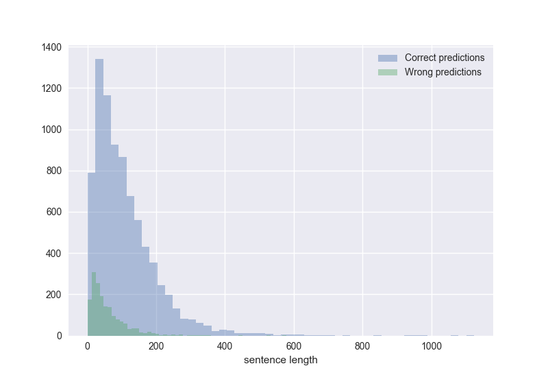
And that’s it! I must say, although throughout this project I have been pushing for higher and higher prediction accuracies, looking at the sentences, I’m fairly impressed that the model got so many sentences right.
There are many more things that can be done that may improve this model. And I may revisit this in the future.